\partial geek

This post is a follow up to my introduction to partial differential equations.

As I mentioned in the other post, it is sometimes not possible to find an expression for the solution to a PDE. So, how can be be sure that the solution even exists? And does it even make sense to talk about the solution if we can’t write it down? Without derailing this post too much, I’ll just say that proving the existance of a solution is an important topic when studying PDE’s. And it makes about as much sense to talk about the solution as talking about \(\pi\) does. While the concept of \(\pi\), the ratio between the circumference of a circle and its diameter, is well defined and exact, we cannot write \(\pi\) down. The best we can do is to write down an approximation. So is the case for many PDEs.

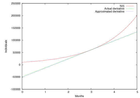
There are several different ways to approximate the solution to a PDE, just as there are several different ways to approximate the value of \(\pi\). The first one I will describe is called the Finite Difference Method (FDM) and is rather intuative. It is usually very easy to implement on a computer, which is why it is frequently used. Before we tackle a full PDE let’s start by looking at the population growth model again, given by \[\dt{N(t)} = rN(t).\]As mentioned, the left hand side is the derivative of \(N(t)\), in other words how much \(N(t)\) will change if \(t\) changes (the slope of \(N(t)\) at time \(t\)). Intuatively we could approximate the derivative by letting \(t\) change slightly and measure how \(N(t)\) changes. We could for instance measure the number of individuals at one time, then again after three months. If we subtract the two numbers we get the change in population, and by dividing this by the change in time between the two measurements we get the approximation of the derivative. Thus, if we count \(N_1\) individuals at some time \(t_1\) and \(N_2\) at some later time \(t_2\) the approximate derivative is given by \[ \dt{N(t)} \approx \frac{N_2 – N_1}{t_2 – t_1}.\]In the general case this approximation is only good in the neighborhood of the interval given by \(t_1\) and \(t_2\). It’s a fairly good approximation at \(t_1\) and \(t_2\) and a very good approximation at the midpoint between \(t_1\) and \(t_2\) (ie after 45 days in the example). This method is called “finite differences”. Let’s see how the example mentioned looks.

Approximated derivative using finite differences at t = 3

In the graph above the derivatives are given by the slope of the tangent lines. Since the population model has a fairly smooth curvature, the derivative is fairly accurately approximated. If we instead measured the population after only a month, we get a much better approximation.

More accurate approximation of derivative at t = 3

Considering it’s name, it’s perhaps not very surprising that this method of approximating the derivative is the main idea behind the finite difference method. We replace the derivatives in the differential equation by finite difference approximations. Let’s apply it to the population model. We’ll approximate the left hand side as follows \[\dt{N(t)} \approx \frac{N(t+\Delta t) – N(t)}{\Delta t},\]where \(\Delta t\) is some small positive number. Note that since \(t_2 = t + \Delta t\) we get \(t_2 – t_1 = t + \Delta t\ – t = \Delta t\). This is called a forward finite difference approximation, because it uses information ahead of \(t\). So our approximation of the model looks like \[\frac{N(t+\Delta t) – N(t)}{\Delta t} = rN(t).\]By rearranging the terms we get \[N(t+\Delta t) = N(t) + \Delta t rN(t).\]Let’s look at this expression more closely. The left hand side is the population count at time \(t + \Delta t\), ie in the future relative to \(t\). On the right hand side we have the population count at time \(t\) pluss the number of offspring at time \(t\) multiplied by the difference in time \(\Delta t\). This means that assuming we know \(N(t)\) we can easily find the approximated population count at the time \(t + \Delta t\). By applying this scheme repeatingly, taking small steps forwards in time, we can form an approximation of \(N(t)\). Since we can calculate the value of \(N(t + \Delta t)\) directly in terms of know values, it is called an explicit scheme. Lets see how our approximation of the population model works out, using the following Python script.

1
2
3
4
5
6
7
8
9
10
11
12
13
14
15
16
17
18
19
20
21
22
23
24
25
26
27
28
29
30
31
32
33
34

from math import exp
 
# N is our population count
# initialize with N0
N0 = 10000
N = N0
 
# r is the reproduction rate per individual per year
r = 0.2
 
# dt is the time step for the simulation
dt = 3.0 / 12.0
 
# current time in years
t = 0
 
# how many years to simulate
tend = 10
 
# iteration count
i = 0
 
while True:
  # output current popluation count,
  # along with analythical solution
  print t, N, N0*exp(r*t)
  # calculate the next value of N
  N_next = N + dt*r*N
  i = i + 1
  t = i*dt
  if t > tend:
    break
  # update current value of N
  N = N_next

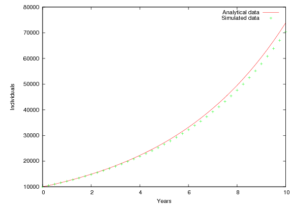
For this simulation \(\Delta t\) was set to three months and \(r = 0.2\). As one can see from the following graph the approximation is very good for a while, but becomes progressively worse.

Comparision between analytical and simulated results

In this case there we had a nice expression for the solution, so finding an approximated solution was a bit pointless. However using the FDM we can find an approximation just as easily even though don’t have a nice expression for the solution. This is why numerical approximations are so powerful, as most interesting problems fall into this latter category.