\partial geek

One of the main features in the upcoming release of LuxRender is proper absorption in transparent media. Before, transparent materials, such as glass, had a single “transmission color”. As a ray entered the material, it was modulated (multiplied) by this color and again if it exited. The problem is that this doesn’t really match how transparent materials work. Thus a long-standing feature request was to implement “proper” absorption. Thanks to jeanphi’s hard work, the time has finally come!

Most transparent materials can be described by the Beer-Lambert law, which gives the transmission of light through a substance as \( T = \frac{I}{I_0} = e^{-\alpha \ell} \). Here \(I\) is the intensity of the light after going through the material, \(I_0\) is the intensity before entering, \(\ell\) is the distance the light traveled through the material and \(\alpha\) is the absorption coefficient. LuxRender works with distances in meters so \(\alpha\) should have units \(m^{-1}\), that is how much is absorbed after one meter.

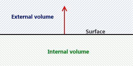
Since absorption is a “volume thing”, as opposed to a “surface thing” like reflectance, objects are now associated with two new volume properties: exterior and interior. These describe the volumes on both sides of the surface of the object. The exterior volume is defined as being on the same side as the surface normal points, while interior is on the opposite side.

Volumes relative to surface normal

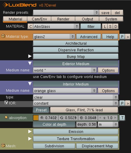
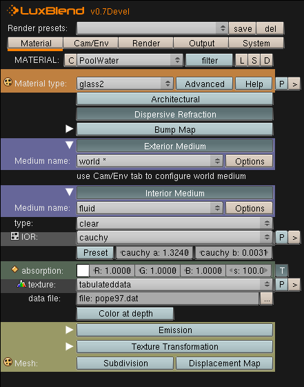
In order to use the new feature you have to use a new material, so far named “glass2”. Instead of the normal material parameters it relies on the mediums in the external and internal volumes. In order to simplify things mediums are named (similar to materials) and can thus be reused. This comes in handy when you have say a glass with a liquid inside it. More on that later. Here’s a screenshot from LuxBlend which shows the new material.

New glass2 media definitions

In the above definition, the exterior medium is set to the special “world” medium, defined in the “Cam/Env” page, which by default is set to air. The interior medium is set to the “clear” volume type, which is the only one supported at the time. It defines a transparent medium with constant index of refraction and absorption according to the Beer-Lambert law. The “Options” button next to the medium name allows you to manage the mediums, such as creating a new one and renaming an existing one.

The absorption definition warrants a closer look. Absorption is in its nature subtractive, meaning that if the medium absorbs a lot of red and green, the object will look blue. And, as mentioned above, the absorption coefficient needs to be specified in “absorption per meter”. In order to make it more intuitive you can use the “Color at depth” button. Enabling this button allows you to specify the color that white light should have after travelling a certain distance through the medium. That is, imagine a white light source behind a slab of your material of the thickness you specify. When you look at the opposite side of the block you should see the color you specify in LuxBlend. LuxBlend converts this information into a suitable absorption coefficient when exporting.

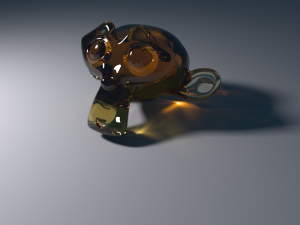
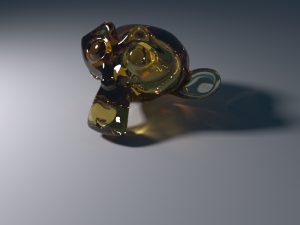
As you can see in the image above, I’ve set the “Color at depth” to a slightly dark orange at a depth of 0.5m. In the image below you can see how the above material looks when applied to the standard Suzanne model which is roughly 2m x 2.5m x 1.5m.

Orange solid glass Suzanne

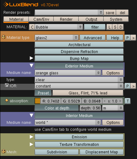
As mentioned LuxRender uses the surface normal to determine if it should use the external or the internal volume at an intersection. This means that you have to be careful to be consistent with your definitions. For example, to add an air bubble inside the glass monkey we make a sphere and place it inside the monkey model. Assuming the normals of the sphere points “out”, we then assign it a material with the internal medium set to “world” (or air), and ensure the external medium is set to the same as the internal medium of the monkey. This is needed because LuxRender doesn’t actually know about the actual volume between the surfaces. Lets take a look at a quick example.

Material definition of air bubble

Of course we could have created a new interior medium, like a liquid for instance with it’s own absorption, but I wanted to keep things simple. As you can see below, the air bubble is clearly visible, both in the lower absorption and in the refractions.

Glass Suzanne with internal air bubble

You can download the glass Suzanne scene here in case you want to play with it yourself.

Physically based data for physically based rendering

Since LuxRender is physically based, measured data from the real world can easily be applied. Thanks to a new “tabulateddata” texture (note, it might change name), LuxRender can use tabulated data files as input for colors, much in the same way .nk files could be used with the metal material. It ignores any text until it finds a header line or a data line. It then reads until it fails to read a data line. The header line is optional and has the following format:

 wavelength: unit, data: description

The wavelength field indicates which units the wavelengths are given in. Currently it accepts the following units: nm, um, eV, cm-1. The data field is currently ignored, so you can write anything for the description. If no header is found it assumes that the wavelength unit is nm. A data line consists of two floating point numbers per line (any additional numbers or data is ignored). Here is an example file.

wavelength: nm	data: absorption (1/cm)
380	0.0001137
500	0.000204
600	0.002224
720	0.01231

Data is linearly interpolated between the samples. The bottom line is that the tabulateddata texture can read lots of data files with little or no modifications. It’s worth noting that the absorption values in the above file has units of \( \text{cm}^{-1} \), while LuxRender expects the absorption to be in units of \( \text{m}^{-1} \).  Thus we need to scale up the absorption by a factor of 100. You can use the “s” field by the absorption color in LuxBlend to do this (see screenshot below).

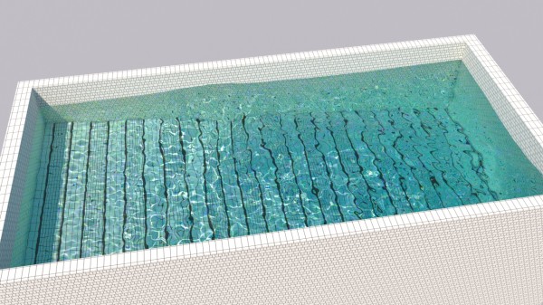
In order to show the power and beauty of using measured data, I made a small pool scene in blender with realistic dimensions. The pool model is about 7.5m x 3.5m and 2.5m at the deepest. I then found a page named Optical Absorption of Water Compendium which has several data files containing measured absorption of seawater. I opted for using the Pope and Fry ’97 data set, which covered the entire visible spectrum.

Another quick search led me to the Index of Refraction of Water page, where I found measured values for the IOR of seawater. Since the page only listed a few data points, all well inside the visible spectrum, I decided to fit the data to Cauchy’s equation. The wavelength-dependent parameter in Cauchy’s equation is given as \( \frac{1}{\lambda^2} \) where the wavelength \( \lambda \) is in micrometers. Converting the wavelengths from the page into this format allowed me to perform a linear fit, yielding the two coefficients: \( A = 1.32401 \) and \( B = 0.00307694 \). These can the be entered into a “cauchy” IOR texture in LuxBlend. Below is the material setup for the water in the pool scene.

Definition of the water material for the pool scene

As you can see I have enabled dispersion which utilizes the “cauchy” IOR texture. What remains is to define the material for the pool walls, where I used a simple diffuse material. Note that the wall material does not need to have any mediums defined, LuxRender will automatically do the right thing here since the walls aren’t transparent. Below you can see how this turned out.

Physically based pool scene

Jump in and enjoy 🙂